Complexity Classes and their Graphs: BEHIND THE SCENES!

Welcome

---

Hi! Welcome to this section on Complexity Classes and their Graphs. First of all, congratulations on these weeks of hard work!! : ) You’ve done a fantastic job and we’re so glad you’ve come this far.

---

• You learned in lecture that algorithms have different running times and how the orders of growth tell you how efficient an algorithm is, given very large inputs. The order of growth is an approximation, an upper bound on how much an algorithm could take to run, the worst-case scenario.
• We will first have a quick introduction to 2-D graphs and then we’ll discuss and illustrate the logic behind each complexity you’ve learned (constant, logarithmic, linear, loglinear, polynomial and exponential).

---

The Graph

The complexity classes are represented with a graph.

Graphs have two axes:

• The X-axis, a horizontal line (represented below with an orange line).
• The Y-axis, a vertical line (represented below with a green line).

Each point on the graph has two coordinates, an x-coordinate and a y-coordinate and the point itself is represented as (<x-coordinate>, <y-coordinate>).

• The point where the x-axis and y-axis intersect is the origin, the point (0, 0).
• We start counting positive numbers from the origin to the right on the X-axis and from the origin above on the Y-axis.
• We start counting negative numbers from the origin to the left on the X-axis and from the origin below on the Y-axis. (You can visualize this on the blank graph below the first diagram)

---

X-axis

• In our case, for algorithmic complexity, the numbers on the x-axis represent the size of the input.

Y-axis

• In our case, for algorithmic complexity, the numbers on the y-axis represent the upper bound for the execution time of an algorithm given the input size that corresponds to this y value on the x-axis.

---

---

More on Graphs

A 2-D (2-dimentional) graph is a line (can be a curve).

• Each point on this line has two coordinates (x, y). For our purposes, each input size on the x-axis will have a corresponding y-coordinate, the upper bound on its execution time and will be represented as (<inputSize>, <executionTime>).

On the example below, we have a point that is represented as a very thick point. This point has two coordinates (input1, a).

Let’s check this:

• If we draw a vertical line from the point to the x-axis, we reach input1 (represented as a red bubble for illustration purposes). This input1 for this example is an arbitrary input size.
• If we draw a horizontal line from the point to the y-axis, we reach a.

We’ve determined that this point has these coordinates (input1, a).

The same principles apply for each point on the graph and that’s how we get a continuous line.

---

How to Read a Graph

Since we start at the origin, (0, 0) where the two axes intersect, the numbers on the x-axis and y-axis get larger as we go right and up, respectively.

• If we take two input sizes on the x-axis, the one to the left will be the smallest and the one to the right will be the largest.
• If we take two execution times on the y-axis, the one that is located higher is the largest one and the one below is the smallest one.

In this case we take input1 and input2 (the two red bubbles on the x-axis) and we find their corresponding points on the line (represented as thick points for illustration purposes). These points have a and b as y-coordinates, respectively.

• What the graph is telling us is that input1 is smaller in size than input2 and that input1 takes less time to execute than input2 since its y-coordinate is smaller.

---

---

Complexity Classes in Context!

Now let’s visualize and analyze each one of the algorithmic complexities we will be studying.

---

Constant complexity

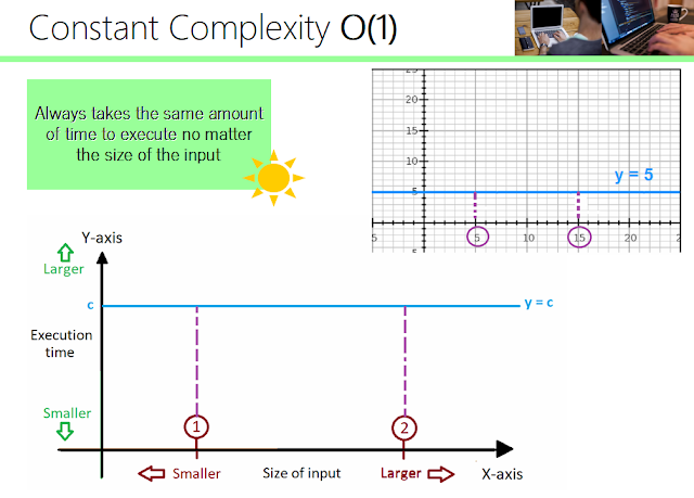
This is our best friend! Algorithms with this complexity are the most efficient. An algorithm with this complexity always takes approximately the same amount of time/steps to execute, no matter the size of the input.

As you can see on the graphs below, we have input1 and input2 (the two red bubbles on the x-axis).

A constant complexity graph is represented as a horizontal line (blue line below) because as the input gets larger, the time required to execute is approximately the same.

On the graph on the top right hand-size corner of the diagram you can see an example of a constant graph y = 5.

---

NOTE: These helper graphs on the top right hand-side corner of the diagrams (provided by graphsketch.com) illustrate how much the y-coordinate changes on each complexity graph when we triple the size of the input. The numbers on the x and y axes (5 and 15 in this case) are not within the context of algorithms. These are general examples of these types of functions represented mathematically)

---

Logarithmic Complexity

This complexity is great as well, the execution time increases slowly with input size. You can see how if we triple the input (5 to 15) the change in y-coordinate (execution time) is very small so the algorithm is very efficient.

---

---

Linear Complexity

Now we go to linear complexity. This complexity starts to be less efficient because if we multiply the input size by a constant (e.g double, triple the size of the input), the algorithm will take double, triple or c times (c a constant) the time it took for n (the initial input size) to execute.

---

---

LogLinear complexity

This complexity start to be inefficient since its the execution time grows faster than linearly. You can see on the graph that if we triple the size of the input (from 5 to 15) the y-coordinate is a little bit more than triple.

---

---

Polynomial Complexity

Algorithms with this complexity are very inefficient. The larger the value of c (the constant to which we raise the size of the input) the longer it takes to execute.

In this case, we have an example where c = 2 so the graph is y = x^2. You can see that the input is squared and that gives us the y-coordinate (time to execute) so the graph grows extremely fast and it illustrates why this algorithm takes too much to execute on large inputs.

---

---

Here you can see some more polynomial graphs. Notice how they grow much faster as we increase the value of c, the exponent.

---

Exponential Complexity

WARNING! Algorithms with exponential complexity take an extremely large amount of time to execute on large inputs.

You can see how the execution time on the graph below grows from a very small number on the y-axis for an input of 5 to more than 30000 when we triple the input size.

Larger the base (c), longer execution time.

---

Here you can see more exponential graphs and how as the base get larger, the execution time grows faster as well.

---

Here are all the graphs used in this tutorial together, so you can see the difference between each complexity class and how their graphs grow with input size.

Hope it helps!

If you have any questions please do not hesitate to ask on the forums or right below this post. Community TAs and your classmates will be there to help you : )

Estefania.